
Artwork by Allison Horst
Introduction
Throughout the years, we become more fluent using R. However, like in any language, use of accurate words (functions in this case) can shorten, clarify, and save a lot of time in communicating code or insights.
The purpose of this post is to summarize a few functions learned the hard way, to be used a reference for me, and maybe allow you to discover some new functions or new use cases for functions you already know.
Data
For demonstrating purposes, we will use data from the tidytuesday project regarding Chocolate Ratings.
chocolate <- readr::read_csv('https://raw.githubusercontent.com/rfordatascience/tidytuesday/master/data/2022/2022-01-18/chocolate.csv')

skimr::skim(chocolate)
| Name | chocolate |
| Number of rows | 2530 |
| Number of columns | 10 |
| _______________________ | |
| Column type frequency: | |
| character | 7 |
| numeric | 3 |
| ________________________ | |
| Group variables | None |
Variable type: character
| skim_variable | n_missing | complete_rate | min | max | empty | n_unique | whitespace |
|---|---|---|---|---|---|---|---|
| company_manufacturer | 0 | 1.00 | 2 | 39 | 0 | 580 | 0 |
| company_location | 0 | 1.00 | 4 | 21 | 0 | 67 | 0 |
| country_of_bean_origin | 0 | 1.00 | 4 | 21 | 0 | 62 | 0 |
| specific_bean_origin_or_bar_name | 0 | 1.00 | 3 | 51 | 0 | 1605 | 0 |
| cocoa_percent | 0 | 1.00 | 3 | 6 | 0 | 46 | 0 |
| ingredients | 87 | 0.97 | 4 | 14 | 0 | 21 | 0 |
| most_memorable_characteristics | 0 | 1.00 | 3 | 37 | 0 | 2487 | 0 |
Variable type: numeric
| skim_variable | n_missing | complete_rate | mean | sd | p0 | p25 | p50 | p75 | p100 | hist |
|---|---|---|---|---|---|---|---|---|---|---|
| ref | 0 | 1 | 1429.80 | 757.65 | 5 | 802 | 1454.00 | 2079.0 | 2712 | ▆▇▇▇▇ |
| review_date | 0 | 1 | 2014.37 | 3.97 | 2006 | 2012 | 2015.00 | 2018.0 | 2021 | ▃▅▇▆▅ |
| rating | 0 | 1 | 3.20 | 0.45 | 1 | 3 | 3.25 | 3.5 | 4 | ▁▁▅▇▇ |
Wrangling
1 - separate_rows()
As you may have noticed, the most memorable characteristics of a chocolate are organized in a string with multiple characteristics separated by commas.
 [1] "dominate cocoa notes"          "muted, nutty"
 [3] "intense, sweet, brownie"       "creamy, complex, coffee"
 [5] "sandy, tobacco, molasses"      "strawberry, butterscotch, off"
 [7] "nutty, off, roasty, fatty"     "astringent, smomkey cocoa"
 [9] "grassy, earthy, coffee"        "gritty, sticky, smoke,hammy"
Often, we would like to “unlist” those characteristics, maybe to understand how people describe chocolate. One way of doing this is using separate(). However, this poses an inconvenience when the number of objects in the list is unknown or variable. ‘separate_rows()’ simplifies the process.
chocolate_separated <- chocolate %>%
    select(most_memorable_characteristics, rating) %>%
    separate_rows(most_memorable_characteristics, sep = ", ")

chocolate_separated
# A tibble: 6,927 x 2
   most_memorable_characteristics rating
   <chr>                           <dbl>
 1 rich cocoa                       3.25
 2 fatty                            3.25
 3 bready                           3.25
 4 cocoa                            3.5
 5 vegetal                          3.5
 6 savory                           3.5
 7 cocoa                            3.75
 8 blackberry                       3.75
 9 full body                        3.75
10 chewy                            3
# ... with 6,917 more rows
This makes finding the most used descriptions easy.
chocolate_words <- chocolate_separated %>%
    group_by(most_memorable_characteristics) %>%
    summarize(n = n(), avg_rating = mean(rating))

chocolate_words %>%
    top_n(10, n)
# A tibble: 10 x 3
   most_memorable_characteristics     n avg_rating
   <chr>                          <int>      <dbl>
 1 cocoa                            242       3.38
 2 creamy                           186       3.47
 3 earthy                           187       3.03
 4 fatty                            163       3.08
 5 floral                           143       3.25
 6 nutty                            259       3.29
 7 roasty                           209       3.20
 8 sandy                            164       3.10
 9 spicy                            138       3.30
10 sweet                            264       3.05
2 - filter with if_any(), if_all()
Another common problem is filtering across columns. One neat trick is to use if_any() and if_all(). Suppose we want to filter common words that also have a high avg_rating.
chocolate_words %>%
    filter(if_all(n:avg_rating, ~.x > quantile(.x, 0.75))) %>%
    arrange(desc(avg_rating))
# A tibble: 21 x 3
   most_memorable_characteristics     n avg_rating
   <chr>                          <int>      <dbl>
 1 peanut                             7       3.75
 2 balanced                          16       3.73
 3 raspberry                         13       3.71
 4 mild tart                          4       3.69
 5 rich choco                         4       3.69
 6 robust                             4       3.69
 7 long                              10       3.62
 8 blackberry                        11       3.61
 9 delicate                          12       3.60
10 dark berry                        17       3.60
# ... with 11 more rows
Or maybe, you want to filter words that are either common or have high average rating.
# A tibble: 366 x 3
   most_memorable_characteristics     n avg_rating
   <chr>                          <int>      <dbl>
 1 sweet                            264       3.05
 2 nutty                            259       3.29
 3 cocoa                            242       3.38
 4 roasty                           209       3.20
 5 earthy                           187       3.03
 6 creamy                           186       3.47
 7 sandy                            164       3.10
 8 fatty                            163       3.08
 9 floral                           143       3.25
10 spicy                            138       3.30
# ... with 356 more rows
These functions help a lot when dealing with many columns of similar properties. Especially if you work with questionnaires or questionnaires scores and want to see if multiple categories are true.
3 - condition with !x %in% y
One of the functions I love and use frequently is %in%. However, its negation is often not intuitive. Some people use packages to allow for a %nin% function, (others build their own function)[https://twitter.com/vishal_katti/status/1111712316649689088]. Maybe it is because I learned R before SQL, but I prefer not writing a function or using a package for just one function when I can use an existing syntax.
chocolate %>%
    count(company_location, sort = T) %>%
    filter(!company_location %in% c("U.S.A.", "Canada", "France"))
# A tibble: 64 x 2
   company_location     n
   <chr>            <int>
 1 U.K.               133
 2 Italy               78
 3 Belgium             63
 4 Ecuador             58
 5 Australia           53
 6 Switzerland         44
 7 Germany             42
 8 Spain               36
 9 Denmark             31
10 Japan               31
# ... with 54 more rows
4 - count(.drop = F) explicitly
All credit to Shannon Pileggi on this one. This allows to explicitly show all levels of a factor (or combinations of factors) when counting, even if it has zero occurrences.
chocolate %>%
    mutate(across(c(company_location, country_of_bean_origin), factor)) %>%
    count(company_location, country_of_bean_origin, sort = T, .drop = F) %>%
    tail()
# A tibble: 6 x 3
  company_location country_of_bean_origin     n
  <fct>            <fct>                  <int>
1 Wales            Trinidad                   0
2 Wales            U.S.A.                     0
3 Wales            Uganda                     0
4 Wales            Vanuatu                    0
5 Wales            Venezuela                  0
6 Wales            Vietnam                    0
5 - complete() explicitly
This one is similar to the count(.drop = F) trick, but allows us to fill the other columns in missing categories with whatever relevant values. Here for example it would be reasonable to fill the count with 0, but the rating with NA.
set.seed(2022)

chocolate_sample <- chocolate %>%
    group_by(company_location, country_of_bean_origin) %>%
    summarize(n = n(), avg_rating = mean(rating), .groups = "drop") %>%
    sample_n(2)

chocolate_sample
# A tibble: 2 x 4
  company_location country_of_bean_origin     n avg_rating
  <chr>            <chr>                  <int>      <dbl>
1 Italy            Madagascar                 6       3.25
2 U.S.A.           Honduras                  15       3.33
chocolate_sample %>%
complete(company_location, country_of_bean_origin,
fill = list(n = 0, rating = NA_real_))
# A tibble: 4 x 4
  company_location country_of_bean_origin     n avg_rating
  <chr>            <chr>                  <dbl>      <dbl>
1 Italy            Honduras                   0      NA
2 Italy            Madagascar                 6       3.25
3 U.S.A.           Honduras                  15       3.33
4 U.S.A.           Madagascar                 0      NA
Visualizations
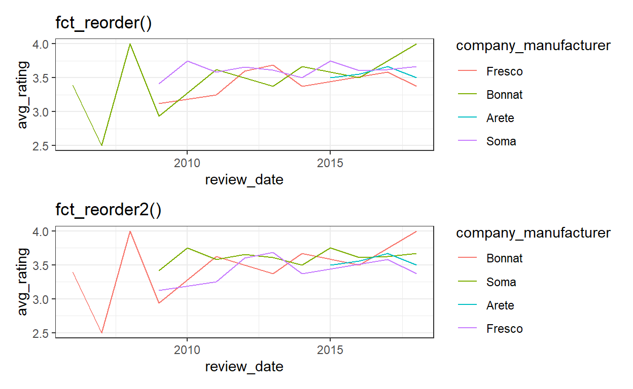
Whenever visualizing multiple time-series, arranging the legend can be a pain. the usual fct_reorder() does not deliver here. No more. Notice the difference in the order.
6 - fct_reorder2()
chocolate_rating_by_year_company <- chocolate %>%
    group_by(company_manufacturer) %>%
    filter(n() >= 30, review_date <= 2018) %>%
    group_by(company_manufacturer, review_date) %>%
    summarize(avg_rating = mean(rating), .groups = "drop")

chocolate_rating_by_year_company
# A tibble: 30 x 3
   company_manufacturer review_date avg_rating
   <chr>                      <dbl>      <dbl>
 1 Arete                       2015       3.5
 2 Arete                       2016       3.56
 3 Arete                       2017       3.67
 4 Arete                       2018       3.5
 5 Bonnat                      2006       3.39
 6 Bonnat                      2007       2.5
 7 Bonnat                      2008       4
 8 Bonnat                      2009       2.94
 9 Bonnat                      2011       3.62
10 Bonnat                      2013       3.38
# ... with 20 more rows
g1 <- chocolate_rating_by_year_company %>%
mutate(company_manufacturer = fct_reorder(company_manufacturer, avg_rating)) %>%
ggplot(aes(review_date, avg_rating, color = company_manufacturer)) +
geom_line() +
labs(title = "fct_reorder()")
g2 <- chocolate_rating_by_year_company %>%
mutate(company_manufacturer = fct_reorder2(.f = company_manufacturer,
.x = review_date,
.y = avg_rating)) %>%
ggplot(aes(review_date, avg_rating, color = company_manufacturer)) +
geom_line() +
labs(title = "fct_reorder2()")
g1 / g2
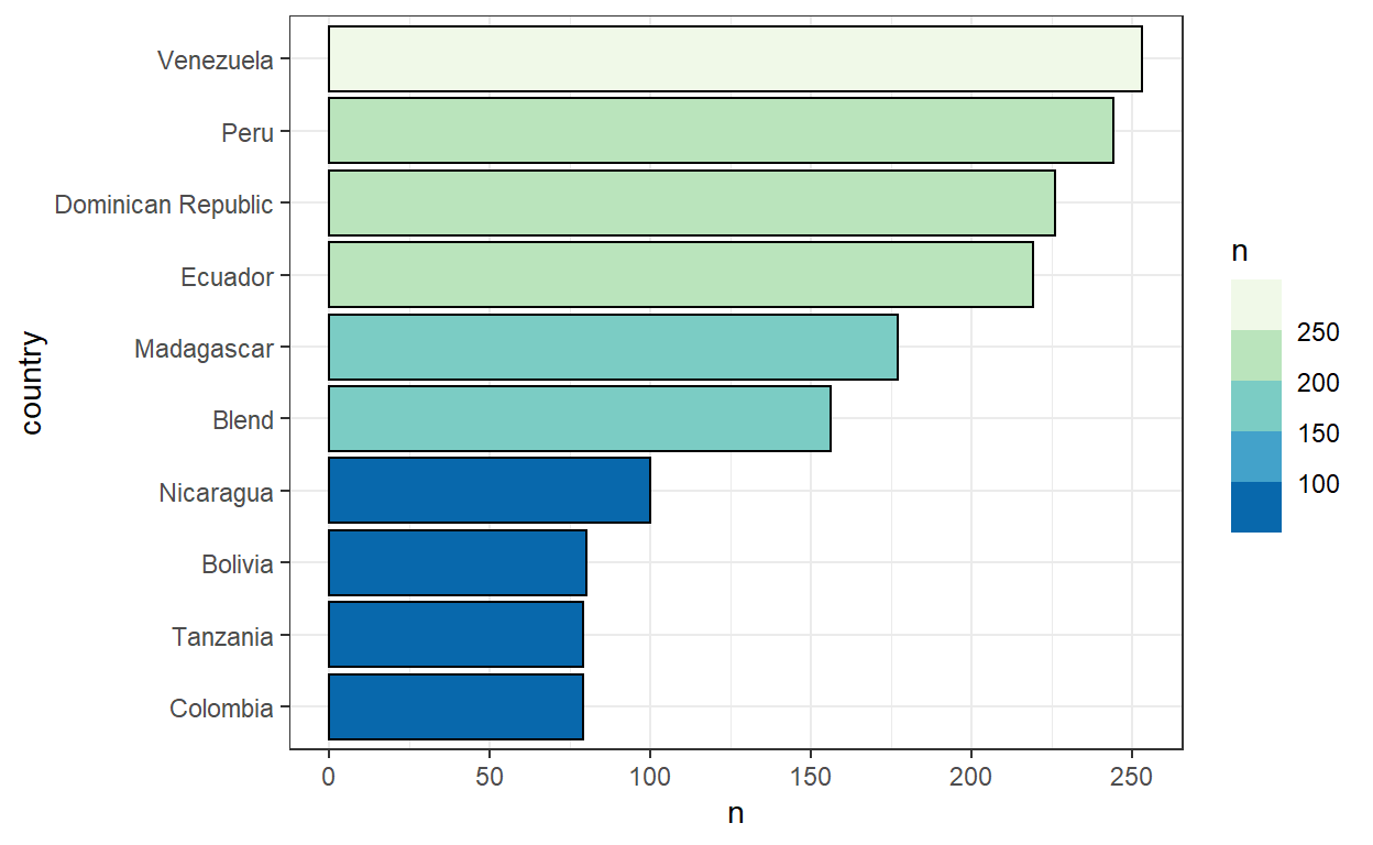
7 - scale_fill_fermenter()
Often, I use a continuous variable as the fill/color aesthetics but I prefer it would be binned by steps. scale_fill_fermenter() is from the same family of scale_fill_brewer() and scale_fill_distiller(), but allows binning of the continuous scale and allows to understand whether a value is in a range more easily.
chocolate %>%
    count(country_of_bean_origin, sort = T) %>%
    head(10) %>%
    mutate(country = fct_reorder(country_of_bean_origin, n)) %>%
    ggplot(aes(n, country, fill = n)) +
    geom_col(color = "black") +
    scale_fill_fermenter(palette = 4, breaks = seq(0,300, 50))
Interactive coding
8 - mid-pipe print()
After building a massive piping system, sometimes you want to print an intermediate value to check that everything performs as expected. Just pipe, print, and pipe again. When you finish, you could just Ctrl + D those lines.
chocolate %>%
    print() %>%
    select(company_manufacturer, rating) %>%
    print() %>%
    group_by(company_manufacturer) %>%
    summarize(n = n(), avg_rating = mean(rating))
# A tibble: 2,530 x 10
     ref company_manufacturer company_location review_date
   <dbl> <chr>                <chr>                  <dbl>
 1  2454 5150                 U.S.A.                  2019
 2  2458 5150                 U.S.A.                  2019
 3  2454 5150                 U.S.A.                  2019
 4  2542 5150                 U.S.A.                  2021
 5  2546 5150                 U.S.A.                  2021
 6  2546 5150                 U.S.A.                  2021
 7  2542 5150                 U.S.A.                  2021
 8   797 A. Morin             France                  2012
 9   797 A. Morin             France                  2012
10  1011 A. Morin             France                  2013
# ... with 2,520 more rows, and 6 more variables:
#   country_of_bean_origin <chr>,
#   specific_bean_origin_or_bar_name <chr>, cocoa_percent <chr>,
#   ingredients <chr>, most_memorable_characteristics <chr>,
#   rating <dbl>
# A tibble: 2,530 x 2
   company_manufacturer rating
   <chr>                 <dbl>
 1 5150                   3.25
 2 5150                   3.5
 3 5150                   3.75
 4 5150                   3
 5 5150                   3
 6 5150                   3.25
 7 5150                   3.5
 8 A. Morin               3.5
 9 A. Morin               3.75
10 A. Morin               2.75
# ... with 2,520 more rows
# A tibble: 580 x 3
company_manufacturer n avg_rating
<chr> <int> <dbl>
1 5150 7 3.32
2 A. Morin 26 3.42
3 Acalli 4 3.56
4 Adi aka Fijiana (Easy In Ltd) 4 3.25
5 Aelan 4 2.75
6 Aequare (Gianduja) 2 2.88
7 Ah Cacao 1 3
8 Akesson's (Pralus) 3 3.08
9 Alain Ducasse 6 2.83
10 Alexandre 4 3.5
# ... with 570 more rows9 - identity()
This one is a frustration-saver. When working with pipes, it could be exhausting to remove the previous line whenever you delete the last line. Add an identity() as the last line, and then you can add/remove all the others without worries.
# A tibble: 580 x 2
company_manufacturer n
<chr> <int>
1 5150 7
2 A. Morin 26
3 Acalli 4
4 Adi aka Fijiana (Easy In Ltd) 4
5 Aelan 4
6 Aequare (Gianduja) 2
7 Ah Cacao 1
8 Akesson's (Pralus) 3
9 Alain Ducasse 6
10 Alexandre 4
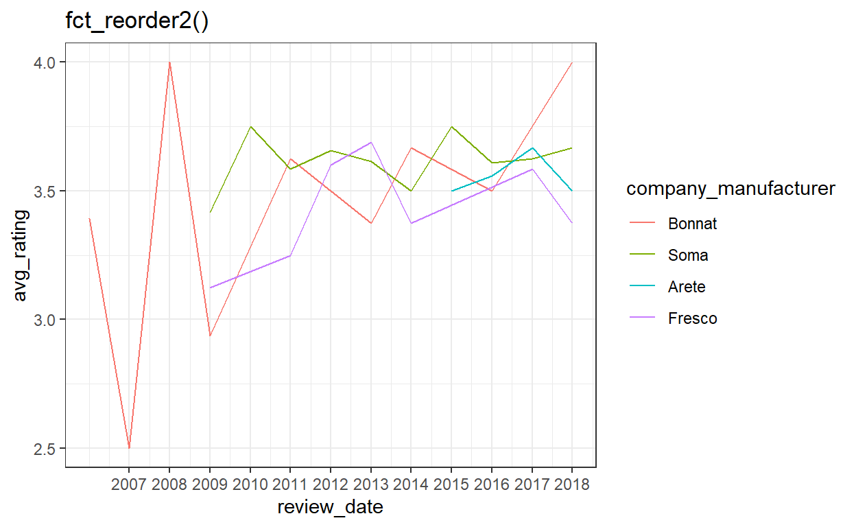
# ... with 570 more rows10 - NULL
This one is actually not a function. It serves the same purpose as identity() but for ggplots.
g2 +
    scale_x_continuous(breaks = seq(2007,2018, 1)) +
    NULL
Summary
As I wrote at the beginning, the purpose of this post was to summarize a few functions learned the hard way, to be used a reference for me, and maybe allow you to discover some new functions or new use cases for functions you already know. What are your secret functions?